Tembo’s Blog


David E. Wheeler
Principal Architect
What’s New on the PGXN v2 Project
6 min read
Sep 11, 2024


Ry Walker
Founder/CEO
pg_auto_dw: a Postgres extension to build well-formed data warehouses with AI
3 min read
Sep 11, 2024

David E. Wheeler
Principal Architect
To Preload, or Not to Preload
6 min read
Jul 24, 2024


Samay Sharma
CTO
Introducing pg_timeseries: Open-source time-series extension for PostgreSQL
6 min read
May 20, 2024

David E. Wheeler
Principal Architect
What’s Happening on the PGXN v2 Project
4 min read
Apr 3, 2024

Vinícius Miguel
Software Engineer
Announcing support for Postgres 14 and 16
2 min read
Mar 15, 2024


Steven Miller
Founding Engineer
Announcing Tembo CLI: Infrastructure as code for the Postgres ecosystem
3 min read
Mar 8, 2024
David E. Wheeler
Principal Architect
The Jobs to be Done by the Ideal Postgres Extension Ecosystem
6 min read
Feb 21, 2024


Binidxaba
Community contributor
Pgvector vs Lantern part 2 - The one with parallel indexes
3 min read
Feb 5, 2024


Adam Hendel
Founding Engineer
Automate vector search in Postgres with any Hugging Face transformer
6 min read
Feb 2, 2024

David E. Wheeler
Principal Architect
Presentation: Introduction to the PGXN Architecture
2 min read
Feb 1, 2024

Adam Hendel
Founding Engineer
How we built our customer data warehouse all on Postgres
9 min read
Jan 25, 2024

Samay Sharma
CTO
PGXN creator David Wheeler joins Tembo to strengthen PostgreSQL extension ecosystem
4 min read
Jan 22, 2024
Binidxaba
Community contributor
Benchmarking Postgres Vector Search approaches: Pgvector vs Lantern
6 min read
Jan 17, 2024

Darren Baldwin
Engineer
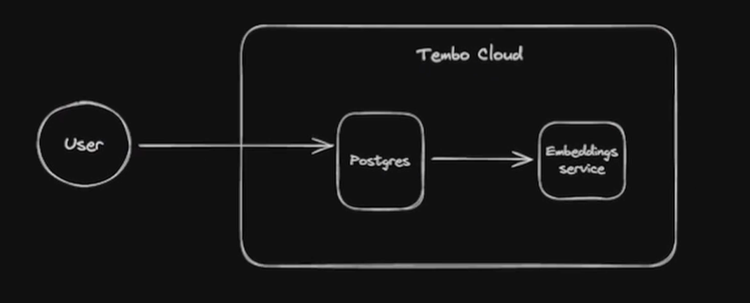
Secure Embeddings in Postgres without the OpenAI Risk
4 min read
Jan 3, 2024

Jay Kothari
Software Engineering Intern
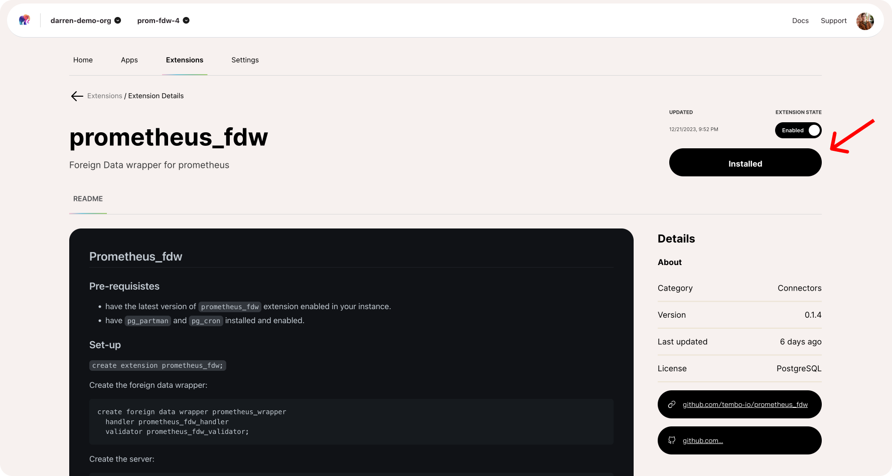
Introducing prometheus_fdw: Seamless Monitoring in Postgres
3 min read
Dec 22, 2023

Binidxaba
Community contributor
Vector Indexes in Postgres using pgvector: IVFFlat vs HNSW
10 min read
Nov 14, 2023
Steven Miller
Founding Engineer
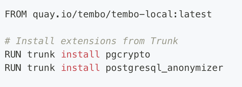
Anonymized dump of your Postgres data
3 min read
Oct 24, 2023
Binidxaba
Community contributor
Unleashing the power of vector embeddings with PostgreSQL
8 min read
Oct 18, 2023
Jay Kothari
Software Engineering Intern
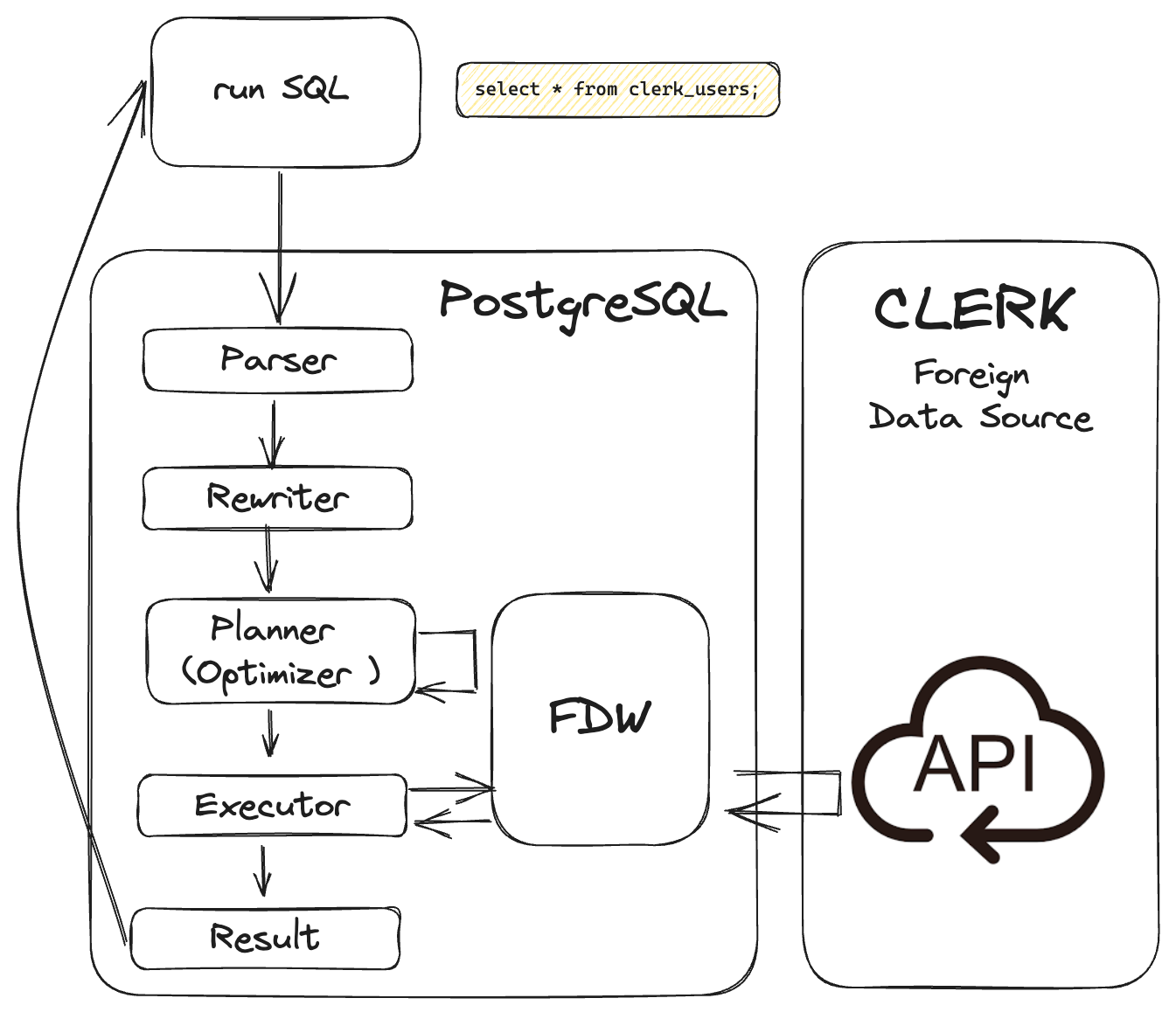
Unlocking value from your Clerk User Management platform with Postgres
5 min read
Oct 3, 2023

Steven Miller
Founding Engineer
Version History and Lifecycle Policies for Postgres Tables
17 min read
Sep 29, 2023
Binidxaba
Community contributor
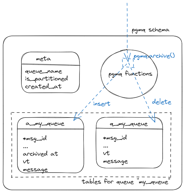
Anatomy of a Postgres extension written in Rust: pgmq
11 min read
Sep 28, 2023

Steven Miller
Founding Engineer
Enter the matrix: the four types of Postgres extensions
12 min read
Sep 14, 2023
Binidxaba
Community contributor
Using pgmq with Python
5 min read
Aug 24, 2023

Adam Hendel
Founding Engineer
Introducing pg_later: Asynchronous Queries for Postgres, Inspired by Snowflake
4 min read
Aug 16, 2023
Adam Hendel
Founding Engineer
Introducing PGMQ: Simple Message Queues built on Postgres
5 min read
Aug 3, 2023
