2 posts tagged with "pgvector"

Image credit: Generated with Bing Image Creator

In databases, indexes are data structures that speed up finding specific values in a table column. The analogous task in vector databases consists of finding the (approximate) nearest-neighbors of a given vector. So, to accomplish this task fast, we can similarly create specialized vector indexes.

But, speeding up a query is not just about blindly creating an index. When deciding whether to create one or more indexes on a table, several factors need to be considered—for example, the size of the tables, whether the table is modified frequently, how the table is used in queries, and so on. Similar considerations apply to vector indexes.

In today's post, let us explore vector indexes and their tradeoffs in the context of Postgres and Pgvector. In particular, let us compare their build time, size, and speed, and, based on that, derive some guidelines to decide which one to choose for a given application.

Indexes in Pgvector​

Pgvector is an open-source Postgres extension for similarity search. It allows for exact and approximate nearest-neighbor search. In particular, for ANN it offers two types of indexes: IVFFlat and HNSW. Let us briefly discuss them.

IVFFlat​

The IVFFlat (Inverted File with Flat Compression) index works by dividing the vectors in the table into multiple lists. The algorithm calculates a number of centroids and finds the clusters around those centroids. So, there is a list for each centroid, and the elements of these lists are the vectors that make up its corresponding cluster.

When searching for the K nearest vectors, instead of calculating the distance to all vectors, the search space is narrowed to only a subset of the lists, thus reducing the number of computations. Which lists are the candidates? The ones whose centroid is closer to the search vector.

IVFFlat generates lists based on clusters.

So, we can infer that the effectiveness of the index depends on two parameters: the number/size of the lists and the number of lists that need to be examined during the search (aka probes).

In pgvector, these two parameters are selected in two distinct moments. First, the number of lists is chosen when creating the index, for example:

CREATE INDEX ON items USING ivfflat (embedding vector_cosine_ops) WITH (lists = 1000)

Second, the number of lists to be explored is established during execution, e.g.:

SET ivfflat.probes = 32

The pgvector documentation suggests the following:

Choose an appropriate number of lists - a good place to start is rows / 1000 for up to 1M rows and sqrt(rows) for over 1M rows

When querying, specify an appropriate number of probes (higher is better for recall, lower is better for speed) - a good place to start is sqrt(lists)

So, imagine that we have a dataset of 1M vectors. With the parameters above, pgvector would generate 1,000 lists of approximately 1,000 vectors. When executing a query, it would only query ~32 of such lists and execute ~32,000 comparisons to find the closest neighbors to a search vector. That is, only 0.032X compared to a full scan.

Of course, you can choose different parameters to achieve the desired recall. More on that later in this post.

HNSW​

The Hierarchical Navigable Small Worlds (HNSW) index creates a graph with multiple layers. The nodes in the graph represent vectors, and the links represent distances. Finding the ANN consists of traversing the graph and looking for the shorter distances.

We can think of these layers as different zoom levels of the graph. Zooming out, we see a few nodes (vectors) and links. But as we zoom in, we see more and more nodes and more and more links.

The traversal of the graph resembles a skip list in that if no more candidate nodes are found in the current layer of the graph, the search continues in the next layer (zoom in), where more links should exist.

HNSW creates a graph with multiple layers

For HNSW, two tuning parameters are decided at creation time: the maximum number of connections per layer (m) and the size of the dynamic candidate list for constructing the graph (ef_construction):

CREATE INDEX ON items USING hnsw (embedding vector_cosine_ops) WITH (m = 16, ef_construction = 64)

A bigger value for m means that each node would have more links in each layer of the graph. A big m affects negatively during query time since more connections need to be checked, but it also improves recall.

ef_construction is also used during the build phase of the index, and it indicates the entry points in layer i+1. That means that bigger values would lead to heavier indexes.

Pgvector does not mention any particular recommendation for HNSW, but the defaults are m=16 and ef_construction=64.

Another parameter, ef_search, determines the size of the dynamic candidate list of vectors. In pgvector, the default is ef_search=40, but can be modified as follows at query time:

SET hnsw.ef_search = 100;

Impact of Approximation on Recall​

In the previous sections, I mentioned a couple of times that the build parameters affect recall. What do we mean by that?

Well, Recall measures how many retrieved neighbors are indeed in the true kNN group. For example, a recall of 1.0 means that all calculated neighbors are really the closest. Whereas a recall of 0.5 means that only half of the computed neighbors are the closest. Recall is an important metric because it helps measure the approximation errors and tune the index parameters.

IVFFlat and HNSW are approximate indexes that work with heuristics. That means that there could be errors in their search results.

Take IVFFlat as an example. When deciding which lists to scan, the decision is taken based on the distance to the centroid of the list. Depending on the data and the tuning parameters, the closest vector to the search vector could correspond to a list that was not selected for probing, thus reducing the accuracy of the result.

One way to mitigate this problem and boost recall is to increase the number of lists to probe. But that, of course, would incur a performance penalty. So, improving the recall is not for free, and careful evaluation and tuning of the parameters is paramount.

IVFFlat vs HNSW in the pgvector arena​

Now, let us examine the two types of indexes quantitatively. We will use the ANN benchmark, which we modified to have both algorithms available.

For pgvector, the benchmark creates a table with a vector column, taking the chosen dataset and inserting the items into the table. Then, it builds the selected type of index, and after that, it executes a bunch of queries. The dataset contains both train and test data. The benchmarking program uses the test data to evaluate the recall for each algorithm.

For this comparison, let us use a small dataset of around 1M vectors of 50 dimensions. The test set consists of 10K queries, and we want to obtain the 10 nearest neighbors.

The aspects that we want to evaluate are:

• Build Time
• Size
• Recall
• Speed

For these experiments, let us ask ourselves: How are the different parameters affected if I want a recall of X? In particular, let us set a recall of 0.998.

In pgvector, such recall is achieved with the following settings:

Build Time​

For the chosen parameters, IVFFlat indexes can be created quicker (128 seconds) compared to HNSW (4065 seconds). HNSW creation is almost 32X slower.

Size​

In terms of index size, IVFFlat is again the winner. For a recall of 0.998, IVFFlat requires around 257MB, whereas HNSW requires about 729MB. HNSW requires 2.8X more space.

Speed​

It is in speed where HNSW shines. With a recall of 0.998, HNSW can achieve a throughput of 40.5 QPS, whereas IVFFlat can only execute 2.6 QPS. HNSW is 15.5X better in this aspect.

Recall vs Index Updates​

Another weakness of the IVFFlat index is that it is not resilient to index updates in terms of recall. The reason for that is that the centroids are not recalculated. So, the different regions in the vector space remain the same if vectors are added or removed. If, after a series of updates, the real centroids (if they were recomputed) are different, the previous mapping would be less effective, leading to a worse recall.

In fact, in psql you will get the following messages if you attempt to create an IVFFlat index when there are only a few rows in the table:

postgres=# CREATE TABLE items (id bigserial PRIMARY KEY, embedding vector(3));
CREATE TABLE         

postgres=# INSERT INTO items (embedding) VALUES ('[1,2,3]'), ('[4,5,6]');
INSERT 0 2

postgres=# CREATE INDEX ON items USING ivfflat (embedding vector_l2_ops) WITH (lists = 100);
NOTICE:  ivfflat index created with little data
DETAIL:  This will cause low recall.
HINT:  Drop the index until the table has more data.
CREATE INDEX

postgres=# drop index items_embedding_idx;
DROP INDEX

The solution to this problem would be to recalculate the centroids and the lists... which effectively means rebuilding the index.

HNSW doesn't show that:

postgres=# CREATE INDEX ON items USING hnsw (embedding vector_l2_ops);
CREATE INDEX

To exercise this behavior, I modified the benchmark to set up the database as follows:

1. Insert 1/100 of the training dataset
2. Build the index
3. Insert the rest of the training dataset
4. Execute the queries using the test dataset

For the chosen parameters, we can see that the recall is more sensitive to index updates for IVFFlat. For HNSW, the change is negligible.

Picking the right index for your use case​

As a quick summary, these were there results that we obtained from our experiments:

With the results above, we can then make the following recommendations:

• If you care more about index size, then choose IVFFlat.
• If you care more about index build time, then select IVFFlat.
• If you care more about speed, then choose HNSW.
• If you expect vectors to be added or modified, then select HNSW.

Let us see some examples.

Imagine a case of a database of Constellations for Astronomy. Data updates would be infrequent (inverse of guideline #4), so IVFFlat would be a good candidate. The index would remain of modest size (guideline #1) and give good recall by tuning only two parameters.

Let's take another example. Imagine a system of Facial Recognition. You'd likely want a fast response time (guideline #2) with good accuracy. You may also be OK with the size of the index (inverse of guideline #1). So, HNSW would be the best choice.

The case of an IoT Sensor Data Database where read values keep changing (e.g., temperature, position, etc.) would also be a good candidate for HNSW (guideline #4). IVFFlat could not handle the index changes properly.

Finally, imagine a database of vector embeddings obtained from your company's knowledge base to generate a chatbot. If the knowledge base rarely changes (inverse of guideline #4) and rebuilding the index is acceptable (if recall ever degrades) (guideline #3), you may choose IVFFlat.

Wrapping up…​

In this post, we discussed the two types of indexes currently available in pgvector: IVFFlat and HNSW. We discussed their build parameters and how they affect recall.

With the help of a benchmark, we compared the indexes quantitatively in terms of build time, index size, QPS, and recall. We derived some general guidelines for choosing the appropriate index type based on our results.

I invite everyone to try out the benchmarking program, which can be found here, and the modified version, which is here.

What other elements should we consider when choosing a vector index? Let us know your thoughts at @tembo_io.

Appendix​

The experiments in this post were carried out using a machine with the following characteristics:

Language models are like the wizards of the digital world, conjuring up text that sounds eerily human. These marvels of artificial intelligence, such as GPT-3.5, are sophisticated algorithms that have been trained on vast swathes of text from the internet. They can understand context, generate coherent paragraphs, translate languages, and even assist in tasks like writing, chatbots, and more. Think of them as your trusty digital scribe, ready to assist with their textual sorcery whenever you summon them.

If you have used ChatGPT in the past, you probably were able to suspect that the previous paragraph was generated using it. And that's true. See the prompt here.

From the example above, you can witness the eloquence LLMs are capable of. Some people have been shocked so much that they became convinced that these models were sentient. However, in the end, they are nothing but a large, complex series of matrix and vector operations. These matrices and vectors have been trained to represent the semantic meaning of words.

In today's post, we will explore these meaning vectors and how they are related to Postgres. In particular, we are going to play with sentence transformers, vectors, and similarity search. All of that with the help of the pgvector Postgres extension.

Let’s go!

From words to vectors​

Like we said, a vector can represent many things, for example, the position of a character in a 3D video game, the position of a pixel in your screen, the force applied to an object, a color in the RGB space, or even the meaning of a word…

Word embedding refers to the technique by which words can be represented as vectors. These days, the embeddings offered by OpenAI are very popular. However, other alternatives exist, like word2vect, Glove, FastText, and ELMo.

Similarly, entire sentences can be represented as vectors using OpenAI embeddings or SentenceTransformers, for example.

These models can be accessed through libraries for different languages. The following Python snippet shows how to obtain the vector embeddings of three sentences using SentenceTransformer:

from sentence_transformers import SentenceTransformer

model = SentenceTransformer('all-MiniLM-L6-v2')
sentences = ['SentenceTransformers is a Python framework for state-of-the-art sentence, text and image embeddings.',
             'Pgvector is postgres extension for vector similarity search.',
             'Tembo will help you say goodby to database sprawl, and hello to Postgres.']

sentence_embeddings = model.encode(sentences)

for sentence, embedding in zip(sentences, sentence_embeddings):
    print("Sentence:", sentence)
    print("Embedding:", embedding)
    print("")

The mind-blowing part is that words and sentences with a similar meaning will have similar vectors. This characteristic is the basis of a search technique called similarity search, where we simply find the nearest embedding vectors to find texts that are similar to our query.

Postgres meets Language Models​

Models are great at generating content that seems credible, as shown earlier. However, you may have experienced cases where ChatGPT hallucinates answers or delivers out-of-date information. That's because LLMs are pre-trained using general data. And, because of that, creating a chatbot based only on the pre-trained data wouldn't be helpful for your customers, for instance.

The concept of RAG (Retrieval-Augmented Generation) acknowledges this limitation.

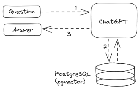
One way of overcoming these problems is to store your company's knowledge base in a database.... preferably in a vector database. You could then query related content and feed that content to the LLM of your preference.

Specialized vector databases include Milvus, Qdrant, Weaviate, and Pinecone. However, you probably want to stick to your Postgres database.

Postgres is not in itself a vector database, but extensions can come to the rescue one more time... This time with pgvector.

Let's use it and explore how we would query related content from a Postgres database.

pgvector: Postgres as a vector database​

pgvector is a Postgres extension that helps work with vectors and stores them in your postgres database. It offers functions for calculating the distance between vectors and for similarity search.

For the following demo, I converted all of Tembo’s blogs into document vectors using the following Python script that uses the langchain framework.

from langchain.document_loaders import TextLoader
from langchain.embeddings import HuggingFaceEmbeddings
from langchain.text_splitter import RecursiveCharacterTextSplitter
from langchain.vectorstores.pgvector import PGVector

import os


CONNECTION_STRING = "postgresql+psycopg2://postgres:password@localhost:5432/vector_db"
COLLECTION_NAME = 'my_collection'

embeddings = HuggingFaceEmbeddings(model_name='all-MiniLM-L6-v2')
text_splitter = RecursiveCharacterTextSplitter(chunk_size = 1000, chunk_overlap = 20)

files = os.listdir('./corpus')

for file in files:
    file_path = f"./corpus/{file}"
    print(f"Loading: {file_path}")
    loader = TextLoader(file_path)
    document = loader.load()
    texts = text_splitter.split_documents(document)
    sentence_embeddings = embeddings.embed_documents([t.page_content for t in texts[:5]])

    db = PGVector.from_documents(
            embedding=embeddings,
            documents=texts,
            collection_name=COLLECTION_NAME,
            connection_string=CONNECTION_STRING)

It basically loads each document and then inserts them into Postgres using the PGVector class. As a result, in my Postgres database called vector_db, I got two tables:

• langchain_pg_collection: contains information about all collections.
• langchain_pg_embedding: contains all the resulting vectors.

The following picture shows part of the contents of (2):

The resulting vectors have 384 dimensions.

Are these sentences similar?​

Let’s now play with these vectors.

Using pgvector we can search content that is similar to a query. For example, we can find content related to postgres 16.

First, we can obtain a vector that represents a query:

from langchain.embeddings import HuggingFaceEmbeddings

embeddings = HuggingFaceEmbeddings(model_name='all-MiniLM-L6-v2')
print embeddings.embed_query(“What is new in postgres 16")

Then we can search vectors stored in the database that are similar to the query vector. The tool for that is cosine distance, which in pgvector is represented with the <=> operator:

SELECT document, 1-(embedding <=> '[<your_vector_here>]') as cosine_similarity
FROM langchain_pg_embedding
ORDER BY cosine_similarity DESC
LIMIT 2;

The above query retrieves vectors/chunks of text ordered by how close they are (in terms of cosine distance) to the query vector. In my case, the most similar chunk of text was:

In case you missed it, Postgres 16 came out last week - and this year it arrived earlier than the last few years. There are many features that I’ve been looking forward to for the last few months and I’m excited to see them get into the hands of users. Before we dive into the specific features of this release, let’s discuss what a Postgres major release actually means.

[postgres-16]

Postgres Releases

The PostgreSQL Global Development Group releases a new major version every year with new features.

In addition, Postgres releases minor versions of each major release every 3 months or so with bug fixes and security fixes. No new features are released in minor versions, and that’s what makes major version releases so exciting as it’s the culmination of about a year’s worth of development work on the project.

Which is an excerpt from Postgres 16: The exciting and the unnoticed.

Let us look at what Postgres is doing behind the scenes, using explain analyze:

Limit  (cost=28.07..28.08 rows=2 width=641) (actual time=1.069..1.071 rows=2 loops=1)
   ->  Sort  (cost=28.07..28.53 rows=181 width=641) (actual time=1.067..1.068 rows=2 loops=1)
         Sort Key: ((embedding <=> '[<your_vector>]'::vector))
         Sort Method: top-N heapsort  Memory: 28kB
         ->  Seq Scan on langchain_pg_embedding  (cost=0.00..26.26 rows=181 width=641) (actual time=0.036..0.953 rows=181 loops=1)
 Planning Time: 0.079 ms
 Execution Time: 1.093 ms
(7 rows)

We can observe that Postgres is sequentially scanning all rows. Then it computes the cosine distance for all those rows and sorts them. Finally, it takes the first two rows.

The sequential scan could be avoided if we had an index. Indeed, we can create one thanks to pgvector, for example:

alter table langchain_pg_embedding alter column embedding type vector(384);

CREATE INDEX ON langchain_pg_embedding  USING ivfflat (embedding vector_cosine_ops) WITH (lists = 100);

 Limit  (cost=5.01..5.11 rows=2 width=641) (actual time=0.175..0.179 rows=1 loops=1)
   ->  Index Scan using langchain_pg_embedding_embedding_idx2 on langchain_pg_embedding  (cost=5.01..13.49 rows=181 width=641) (actual time=0.172..0.175 rows=1 loops=1)
         Order By: (embedding <=> '[<your_vector>]'::vector)
 Planning Time: 0.154 ms
 Execution Time: 0.224 ms
(5 rows)

One thing to keep in mind is that these indexes are used for approximate nearest neighbor search. We’ll explore what that means in a future blog post. Let us know if that would be interesting for you.

Pgvector(ize)?​

Ok, at this point you should now have a sense of what pgvector is, and how to use it together with Python. However, wouldn't it be great if the vectorizing step could happen all within Postgres?

Pg_vectorize is an extension being developed by Tembo that intends to streamline the process of generating vectors from the data in your Postgres tables. It uses a background worker to generate and update the embeddings in batches every N seconds. Also, if you need to find similar vectors, the extension can do that. All within Postgres. Isn't that a cool idea?

I invite you to check out the repository and stay tuned.

To wrap up...​

In this post, we briefly discussed the concept of embeddings, why they are important, and how they can be generated using one of the multiple available libraries. We also explored how to store and query the resulting vectors using Postgres and the pgvector extension.

These concepts are relevant to leveraging a knowledge base in conjunction with LLMs in an emerging technique called RAG. Of course, when implementing a real-life solution, more factors need to be considered, and this post was just an introduction.

I invite everyone to try out pgvector (e.g. using the scripts in this post), and the different operations that it offers. Also, can you think of other uses of pgvector? Let us know your thoughts in @tembo_io.

Disclaimer​

The first paragraph in this blog post was generated using ChatGPT. Here’s the prompt