In today’s world, geographic data stands out for its ability to apply spatial context to collections of points, transforming them into valuable insights. When properly analyzed, these datasets can facilitate predictive modeling and spatial analytics, aiding in everything from disaster response planning to optimizing delivery routes in logistics.
Working with geospatial workloads is not new to Postgres. In fact, its most popular geospatial extension, and certainly one of the most popular in general, PostGIS, has been around since 2001. However, installing PostGIS, its dependencies, related extensions, and loading it up with data is hard for new users of the extension.
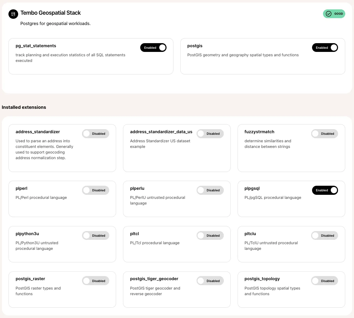
We recently launched the Geospatial Stack to make this easier. The Geospatial Stack is open source and comes pre-packaged with PostGIS and other related extensions, allowing you to perform geospatial analysis without needing to set up another database! You can try it out on your own by using our Kubernetes Operator or deploy it with a single click on Tembo Cloud.
Let’s look at an example of something interesting you could build with Postgres on the Geospatial Stack.
 Figure 1. Snapshot of Tembo’s Geospatial Stack extension overview.
Loading elephant tracking data (and geospatial data in general) into Postgres
Since we’re talking about Postgres, we thought an interesting example to explore would be an elephant’s journey through the forests of Côte d’Ivoire.
The following dataset was gathered by Dr. Mike Loomis and his team and published to the Movebank online database of animal tracking data under the CC0 License.
- Location: Africa, Côte d’Ivoire, Forest Preserve near the village of Dassioko
- Timeframe: 2018 - 2021
- Sample Size: 1
To begin, you can download the dataset here.
By navigating to the local directory containing the dataset, you can load the data into Postgres using your preferred method. There exist numerous tools, such as shp2pgsql and even QGIS, but we opted for ogr2ogr (bundled with GDAL) and executed the command below. If you’re interested in understanding what the parameters mean, or the other options available, please refer to PostGIS’ guide on loading data with ogr2ogr.
ogr2ogr -f "PostgreSQL" \
PG:"dbname<your-database-name> \
user=<your-username> \
password=<your-password> \
host=<your-host>" \
-nln elephant5990 \
-lco PRECISION=NO \
points.shp
Having loaded the dataset into our Tembo instance, we ran the following to explore the database relations:
\d
                    List of relations
 Schema |           Name           |   Type   |  Owner
--------+--------------------------+----------+----------
 public | elephant5990             | table    | postgres
 public | elephant5990_ogc_fid_seq | sequence | postgres
 public | geography_columns        | view     | postgres
 public | geometry_columns         | view     | postgres
 public | pg_stat_statements       | view     | postgres
 public | pg_stat_statements_info  | view     | postgres
 public | spatial_ref_sys          | table    | postgres
(7 rows)
Let’s dive deeper into the schema of the elephant_5990 table.
\d elephant5990
                                        Table "public.elephant5990"
    Column    |         Type         | Collation | Nullable |                    Default
--------------+----------------------+-----------+----------+-----------------------------------------------
 ogc_fid      | integer              |           | not null | nextval('elephant5990_ogc_fid_seq'::regclass)
 timestamp    | character varying    |           |          |
 long         | double precision     |           |          |
 lat          | double precision     |           |          |
 comments     | character varying    |           |          |
 sensor_typ   | character varying    |           |          |
 individual   | character varying    |           |          |
 tag_ident    | character varying    |           |          |
 ind_ident    | character varying    |           |          |
 study_name   | character varying    |           |          |
 utm_east     | double precision     |           |          |
 utm_north    | double precision     |           |          |
 utm_zone     | character varying    |           |          |
 study_tz     | character varying    |           |          |
 study_ts     | character varying    |           |          |
 date         | date                 |           |          |
 time         | character varying    |           |          |
 wkb_geometry | geometry(Point,4326) |           |          |
Indexes:
    "elephant5990_pkey" PRIMARY KEY, btree (ogc_fid)
    "elephant5990_wkb_geometry_geom_idx" gist (wkb_geometry)
Using PostGIS functions to power insights
PostGIS provides functions, indexes and operators to analyze the geospatial attributes in the data. Let’s explore of few interesting insights we could gather from the data set.
ST_Distance
ST_Distance can be used to find the minimum distance between two points. This approach can be extended in a recursive manner to many points.
- As an example, let’s find which hour of the day (24hr format) had the highest average distance traveled (meters) per year?
WITH TimeDistances AS (
    SELECT
        EXTRACT(YEAR FROM timestamp::timestamp) AS year,
        EXTRACT(HOUR FROM timestamp::timestamp) AS hour,
        LAG(wkb_geometry) OVER (ORDER BY timestamp) AS prev_geometry,
        wkb_geometry AS current_geometry
    FROM elephant5990
),
Distances AS (
    SELECT
        year,
        hour,
        ST_Distance(prev_geometry::geography, current_geometry::geography) AS distance
    FROM TimeDistances
    WHERE prev_geometry IS NOT NULL
),
RankedDistances AS (
    SELECT
        year,
        hour,
        AVG(distance) AS avg_distance,
        RANK() OVER (PARTITION BY year ORDER BY AVG(distance) DESC) as rank
    FROM Distances
    GROUP BY year, hour
)
SELECT
    year,
    hour,
    avg_distance
FROM RankedDistances
WHERE rank = 1
ORDER BY year;
 year | hour |    avg_distance
------+------+--------------------
 2018 |   20 | 500.1667879009256
 2019 |   22 | 500.23505130464025
 2020 |   20 | 490.65593160356303
 2021 |   22 | 474.28919337170834
(4 rows)
ST_Contains
ST_Contains checks whether a given geometry “A” contains another geometry “B”. Note that during this exercise we loaded a custom geometry, described in the following section.
- We could ask, throughout the study, how many times did the elephant enter Dassioko Village?
SELECT
COUNT(e.*)
FROM
elephant5990 e,
village v
WHERE
ST_Contains(v.wkb_geometry, e.wkb_geometry);
 count
-------
    47
(1 row)
ST_ConcaveHull, ST_InteriorRingN
ST_ConcaveHull can be used to establish a boundary around a set of points, while also allowing for gaps (known as holes). ST_InteriorRingN can then be used to identify these holes.
- On visual inspection, there appears to be an area of avoidance in the top left region of the dataset. Can this be identified with a query?
WITH Hull AS (
    SELECT ST_ConcaveHull(ST_Collect(e.wkb_geometry), 0.50, true) AS geom
    FROM elephant5990 e
),
Holes AS (
    SELECT
        ST_InteriorRingN(geom, num) AS hole_geom
    FROM
        (SELECT (ST_Dump(geom)).geom, generate_series(1, ST_NumInteriorRings((ST_Dump(geom)).geom)) AS num FROM Hull) AS sub
),
HoleAreas AS (
    SELECT
        hole_geom,
        ST_Area(ST_MakePolygon(ST_AddPoint(hole_geom, ST_StartPoint(hole_geom)))) AS area
    FROM Holes
)
SELECT
    ST_AsBinary(hole_geom) AS wkb_geometry,
    area
FROM HoleAreas
ORDER BY area DESC
LIMIT 1;
          area
------------------------
 0.00016060894274768603
(1 row)
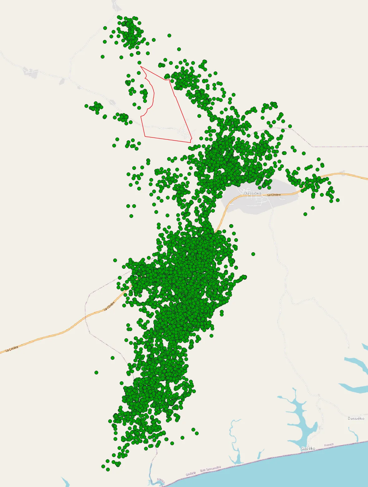
Notice the area’s units are not given. By default this is set to square degrees, but that can be converted to roughly 1.9789 square kilometers. Additionally, this query produces a WKB (Well Known Binary), which we used to generate the QGIS overlay seen in Figure 4. However, due to its character length, we decided not to show the WKB itself.
Visualizing Geospatial Data with QGIS
In addition to running these SQL queries, we could easily overlay this data over maps using QGIS to emit visualizations.
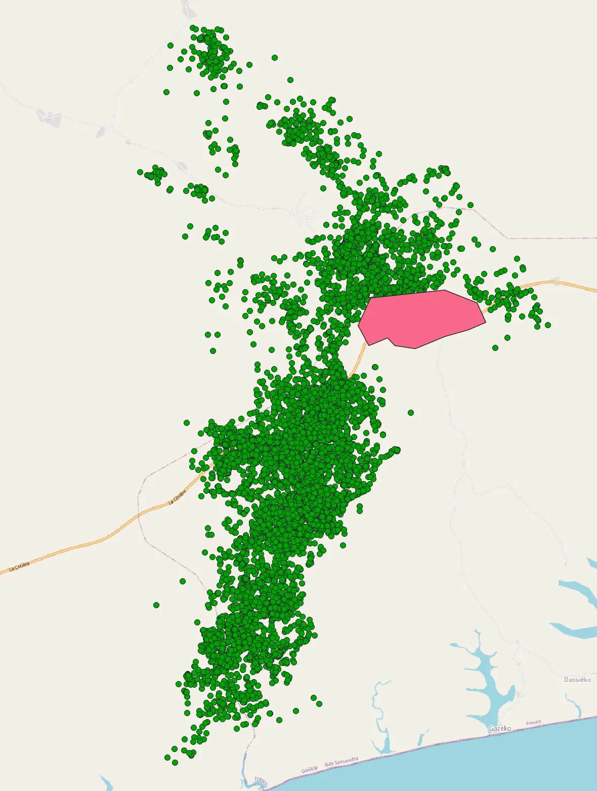
By leveraging QGIS’ OpenStreetMap feature, we can offer real world context to an otherwise meaningless distribution of points. Figure 2 illustrates just such an example. Here we readily see a collection of points, representing the elephant (each point representing measurement captured roughly every two hours). What’s more is that we not only can identify major and minor roads, but the village of Dassioko as well, and what appear to be smaller settlements in its periphery (represented by grey-shaded polygons). Already with this simple overlay, our superficial idea about where the elephant has gone develops into more complex understandings such as:
- Where are the territorial boundaries?
- Where are the areas of clusters and dispersions?
- Are there any sections of roads where the elephant feels most comfortable?
- Are there any identifiable areas of potential human interaction or avoidance?
- And so on!
 Figure 2. QGIS-rendered OpenStreetMap visualization containing elephant tracking data.
QGIS also has built-in features that allow for the creation of custom geometries to visualize and further analyze. As shown above (Figure 2), the OpenStreetMap layer reveals the defined border of Dassioko Village. Not only that, but there are clearly points found within the grey-shaded area, meaning the elephant traveled there. To better quantify this phenomenon, we created a custom geometry and overlayed it (Figure 3). This red-shaded layer helps us answer questions related to the elephant’s behavior in relation to the village.
 Figure 3. QGIS-rendered OpenStreetMap visualization containing elephant tracking data and an overlay geometry representing Dassioko Village. This data is queried above with ST_Contains function.
While the last example involved creating a custom geometry in QGIS and analyzing it in Postgres, this investigative workflow can run in reverse as well. In other words, instead of creating a human-defined geometry and quantifying it with respect to the dataset, we can conduct initial quantifications in Postgres and use the results to generate a QGIS overlay. While the results are not perfect, they are meant as a proof of concept that a potential area of avoidance can be identified with a single query (Figure 4).
 Figure 4. QGIS-rendered OpenStreetMap visualization containing elephant tracking data and an overlay geometry representing a generated potential area of avoidance. This is made possible above with the ST_ConcaveHull and ST_InteriorRingN functions.
Explore Geospatial datasets today!
Using Tembo’s Geospatial Stack, we were able to explore a GPS tracking dataset in a matter of minutes. Though this demonstration focused on the movements of a single elephant, you can use the showcased PostGIS functions for numerous applications to other, business-centric projects like:
- Loading and exploring geospatial datasets
- Insights on time-of-day activity
- Insights on avoidance behavior
- Insights on behavior related to pre-determined areas (zones)
Interested in a more comprehensive guide? Checkout our Geospatial Stack getting started guide.


